
import pandas as pd
import numpy as np
hangover_df = pd.read_csv("hangover_5.csv")
hangover_df.head()
| ID | Night | Theme | Number_of_Drinks | Spent | Chow | Hangover | |
|---|---|---|---|---|---|---|---|
| 0 | 1 | Fri | 1 | 2 | 703 | 1 | 0 |
| 1 | 2 | Sat | 0 | 8 | 287 | 0 | 1 |
| 2 | 3 | Wed | 0 | 3 | 346 | 1 | 0 |
| 3 | 4 | Sat | 0 | 1 | 312 | 0 | 1 |
| 4 | 5 | Mon | 1 | 5 | 919 | 0 | 1 |
pd.DataFrame(hangover_df.columns.values, columns = ["Variables"])
| Variables | |
|---|---|
| 0 | ID |
| 1 | Night |
| 2 | Theme |
| 3 | Number_of_Drinks |
| 4 | Spent |
| 5 | Chow |
| 6 | Hangover |
hangover_df.dtypes
ID                   int64
Night               object
Theme                int64
Number_of_Drinks     int64
Spent                int64
Chow                 int64
Hangover             int64
dtype: object
Convert target variable to categorical.
hangover_df.Hangover = hangover_df.Hangover.astype("category")
Convert some predictors to categorical.
cat_cols = ["Night", "Theme", "Chow"]
hangover_df[cat_cols] = hangover_df[cat_cols].astype('category')
Check data types again.
hangover_df.dtypes
ID                     int64
Night               category
Theme               category
Number_of_Drinks       int64
Spent                  int64
Chow                category
Hangover            category
dtype: object
night_1 = ["Mon", "Tue", "Wed", "Thu", "Fri", "Sat", "Sun"]
night_2 = ["Weekday", "Weekday", "Mid Week", "Mid Week", "Weekend", "Weekend", "Weekend"]

hangover_df["Week_Night_Type"] = hangover_df["Night"].replace(night_1, night_2)
hangover_df.head()
| ID | Night | Theme | Number_of_Drinks | Spent | Chow | Hangover | Week_Night_Type | |
|---|---|---|---|---|---|---|---|---|
| 0 | 1 | Fri | 1 | 2 | 703 | 1 | 0 | Weekend |
| 1 | 2 | Sat | 0 | 8 | 287 | 0 | 1 | Weekend |
| 2 | 3 | Wed | 0 | 3 | 346 | 1 | 0 | Mid Week |
| 3 | 4 | Sat | 0 | 1 | 312 | 0 | 1 | Weekend |
| 4 | 5 | Mon | 1 | 5 | 919 | 0 | 1 | Weekday |
pd.DataFrame(hangover_df.columns.values, columns = ["Variables"])
| Variables | |
|---|---|
| 0 | ID |
| 1 | Night |
| 2 | Theme |
| 3 | Number_of_Drinks |
| 4 | Spent |
| 5 | Chow |
| 6 | Hangover |
| 7 | Week_Night_Type |
Filter the required variables.
hangover_df = hangover_df.iloc[:, [2, 3, 4, 5, 7, 6]]
hangover_df
| Theme | Number_of_Drinks | Spent | Chow | Week_Night_Type | Hangover | |
|---|---|---|---|---|---|---|
| 0 | 1 | 2 | 703 | 1 | Weekend | 0 |
| 1 | 0 | 8 | 287 | 0 | Weekend | 1 |
| 2 | 0 | 3 | 346 | 1 | Mid Week | 0 |
| 3 | 0 | 1 | 312 | 0 | Weekend | 1 |
| 4 | 1 | 5 | 919 | 0 | Weekday | 1 |
| ... | ... | ... | ... | ... | ... | ... |
| 1995 | 1 | 7 | 139 | 1 | Weekday | 1 |
| 1996 | 0 | 3 | 742 | 1 | Mid Week | 1 |
| 1997 | 1 | 7 | 549 | 0 | Weekday | 1 |
| 1998 | 0 | 1 | 448 | 0 | Weekday | 0 |
| 1999 | 1 | 4 | 368 | 1 | Weekday | 1 |
2000 rows × 6 columns
import sklearn
from sklearn.model_selection import train_test_split
sklearn's decision tree function does not work well with strings.
week_night_type_dummies = pd.get_dummies(hangover_df["Week_Night_Type"])
week_night_type_dummies
| Weekend | Weekday | Mid Week | |
|---|---|---|---|
| 0 | 1 | 0 | 0 |
| 1 | 1 | 0 | 0 |
| 2 | 0 | 0 | 1 |
| 3 | 1 | 0 | 0 |
| 4 | 0 | 1 | 0 |
| ... | ... | ... | ... |
| 1995 | 0 | 1 | 0 |
| 1996 | 0 | 0 | 1 |
| 1997 | 0 | 1 | 0 |
| 1998 | 0 | 1 | 0 |
| 1999 | 0 | 1 | 0 |
2000 rows × 3 columns
hangover_df = pd.concat([hangover_df, week_night_type_dummies], axis = 1)
hangover_df.head()
| Theme | Number_of_Drinks | Spent | Chow | Week_Night_Type | Hangover | Weekend | Weekday | Mid Week | |
|---|---|---|---|---|---|---|---|---|---|
| 0 | 1 | 2 | 703 | 1 | Weekend | 0 | 1 | 0 | 0 |
| 1 | 0 | 8 | 287 | 0 | Weekend | 1 | 1 | 0 | 0 |
| 2 | 0 | 3 | 346 | 1 | Mid Week | 0 | 0 | 0 | 1 |
| 3 | 0 | 1 | 312 | 0 | Weekend | 1 | 1 | 0 | 0 |
| 4 | 1 | 5 | 919 | 0 | Weekday | 1 | 0 | 1 | 0 |
Filter required variables. There is no need for 3 dummies for "Week_Night_Type".
pd.DataFrame(hangover_df.columns.values, columns = ["Variables"])
| Variables | |
|---|---|
| 0 | Theme |
| 1 | Number_of_Drinks |
| 2 | Spent |
| 3 | Chow |
| 4 | Week_Night_Type |
| 5 | Hangover |
| 6 | Weekend |
| 7 | Weekday |
| 8 | Mid Week |
# Must be in the same order as the new data

hangover_df = hangover_df.iloc[:,[0, 1, 2, 3, 8, 7, 5]]
hangover_df
| Theme | Number_of_Drinks | Spent | Chow | Mid Week | Weekday | Hangover | |
|---|---|---|---|---|---|---|---|
| 0 | 1 | 2 | 703 | 1 | 0 | 0 | 0 |
| 1 | 0 | 8 | 287 | 0 | 0 | 0 | 1 |
| 2 | 0 | 3 | 346 | 1 | 1 | 0 | 0 |
| 3 | 0 | 1 | 312 | 0 | 0 | 0 | 1 |
| 4 | 1 | 5 | 919 | 0 | 0 | 1 | 1 |
| ... | ... | ... | ... | ... | ... | ... | ... |
| 1995 | 1 | 7 | 139 | 1 | 0 | 1 | 1 |
| 1996 | 0 | 3 | 742 | 1 | 1 | 0 | 1 |
| 1997 | 1 | 7 | 549 | 0 | 0 | 1 | 1 |
| 1998 | 0 | 1 | 448 | 0 | 0 | 1 | 0 |
| 1999 | 1 | 4 | 368 | 1 | 0 | 1 | 1 |
2000 rows × 7 columns
X = hangover_df.drop(columns = ["Hangover"])
y = hangover_df["Hangover"].astype("category")
train_X, valid_X, train_y, valid_y = train_test_split(X, y, test_size = 0.3, random_state = 666)
train_X.head()
| Theme | Number_of_Drinks | Spent | Chow | Mid Week | Weekday | |
|---|---|---|---|---|---|---|
| 817 | 0 | 3 | 644 | 1 | 0 | 0 |
| 1652 | 1 | 9 | 252 | 0 | 0 | 0 |
| 1186 | 1 | 9 | 216 | 0 | 0 | 0 |
| 1909 | 1 | 3 | 196 | 0 | 1 | 0 |
| 87 | 0 | 9 | 519 | 1 | 1 | 0 |
len(train_X)
1400
train_y.head()
817     0
1652    1
1186    1
1909    0
87      1
Name: Hangover, dtype: category
Categories (2, int64): [0, 1]
len(train_y.index)
1400
valid_X.head()
| Theme | Number_of_Drinks | Spent | Chow | Mid Week | Weekday | |
|---|---|---|---|---|---|---|
| 1170 | 0 | 10 | 533 | 1 | 1 | 0 |
| 1852 | 0 | 6 | 257 | 0 | 1 | 0 |
| 1525 | 0 | 2 | 383 | 0 | 0 | 0 |
| 1537 | 0 | 6 | 355 | 0 | 0 | 1 |
| 127 | 1 | 7 | 46 | 1 | 0 | 1 |
len(valid_X)
600
len(valid_y)
600
from sklearn.tree import DecisionTreeClassifier
full_tree = DecisionTreeClassifier(random_state = 666)
full_tree
DecisionTreeClassifier(random_state=666)
full_tree_fit = full_tree.fit(train_X, train_y)
Plot the tree.
from sklearn import tree
Export the top levels for illustration using max_depth. Export the whole tree if max_depth is excluded.
text_representation = tree.export_text(full_tree, max_depth = 5)
print(text_representation)
|--- feature_1 <= 3.50
|   |--- feature_0 <= 0.50
|   |   |--- feature_2 <= 908.00
|   |   |   |--- feature_4 <= 0.50
|   |   |   |   |--- feature_2 <= 828.00
|   |   |   |   |   |--- feature_3 <= 0.50
|   |   |   |   |   |   |--- truncated branch of depth 11
|   |   |   |   |   |--- feature_3 >  0.50
|   |   |   |   |   |   |--- truncated branch of depth 12
|   |   |   |   |--- feature_2 >  828.00
|   |   |   |   |   |--- feature_2 <= 862.50
|   |   |   |   |   |   |--- class: 1
|   |   |   |   |   |--- feature_2 >  862.50
|   |   |   |   |   |   |--- truncated branch of depth 2
|   |   |   |--- feature_4 >  0.50
|   |   |   |   |--- feature_2 <= 497.00
|   |   |   |   |   |--- feature_2 <= 127.50
|   |   |   |   |   |   |--- truncated branch of depth 2
|   |   |   |   |   |--- feature_2 >  127.50
|   |   |   |   |   |   |--- truncated branch of depth 5
|   |   |   |   |--- feature_2 >  497.00
|   |   |   |   |   |--- feature_2 <= 538.50
|   |   |   |   |   |   |--- class: 1
|   |   |   |   |   |--- feature_2 >  538.50
|   |   |   |   |   |   |--- truncated branch of depth 9
|   |   |--- feature_2 >  908.00
|   |   |   |--- feature_5 <= 0.50
|   |   |   |   |--- class: 1
|   |   |   |--- feature_5 >  0.50
|   |   |   |   |--- feature_1 <= 2.50
|   |   |   |   |   |--- feature_2 <= 961.00
|   |   |   |   |   |   |--- class: 0
|   |   |   |   |   |--- feature_2 >  961.00
|   |   |   |   |   |   |--- class: 1
|   |   |   |   |--- feature_1 >  2.50
|   |   |   |   |   |--- class: 1
|   |--- feature_0 >  0.50
|   |   |--- feature_2 <= 983.50
|   |   |   |--- feature_3 <= 0.50
|   |   |   |   |--- feature_4 <= 0.50
|   |   |   |   |   |--- feature_2 <= 38.00
|   |   |   |   |   |   |--- truncated branch of depth 3
|   |   |   |   |   |--- feature_2 >  38.00
|   |   |   |   |   |   |--- truncated branch of depth 8
|   |   |   |   |--- feature_4 >  0.50
|   |   |   |   |   |--- feature_2 <= 759.50
|   |   |   |   |   |   |--- truncated branch of depth 6
|   |   |   |   |   |--- feature_2 >  759.50
|   |   |   |   |   |   |--- class: 0
|   |   |   |--- feature_3 >  0.50
|   |   |   |   |--- feature_1 <= 2.50
|   |   |   |   |   |--- feature_2 <= 133.50
|   |   |   |   |   |   |--- class: 0
|   |   |   |   |   |--- feature_2 >  133.50
|   |   |   |   |   |   |--- truncated branch of depth 13
|   |   |   |   |--- feature_1 >  2.50
|   |   |   |   |   |--- feature_2 <= 46.00
|   |   |   |   |   |   |--- class: 1
|   |   |   |   |   |--- feature_2 >  46.00
|   |   |   |   |   |   |--- truncated branch of depth 8
|   |   |--- feature_2 >  983.50
|   |   |   |--- feature_1 <= 2.50
|   |   |   |   |--- class: 0
|   |   |   |--- feature_1 >  2.50
|   |   |   |   |--- class: 1
|--- feature_1 >  3.50
|   |--- feature_1 <= 6.50
|   |   |--- feature_3 <= 0.50
|   |   |   |--- feature_4 <= 0.50
|   |   |   |   |--- feature_2 <= 338.00
|   |   |   |   |   |--- feature_2 <= 272.50
|   |   |   |   |   |   |--- truncated branch of depth 13
|   |   |   |   |   |--- feature_2 >  272.50
|   |   |   |   |   |   |--- class: 1
|   |   |   |   |--- feature_2 >  338.00
|   |   |   |   |   |--- feature_2 <= 544.00
|   |   |   |   |   |   |--- truncated branch of depth 8
|   |   |   |   |   |--- feature_2 >  544.00
|   |   |   |   |   |   |--- truncated branch of depth 14
|   |   |   |--- feature_4 >  0.50
|   |   |   |   |--- feature_2 <= 864.00
|   |   |   |   |   |--- feature_2 <= 167.50
|   |   |   |   |   |   |--- truncated branch of depth 5
|   |   |   |   |   |--- feature_2 >  167.50
|   |   |   |   |   |   |--- truncated branch of depth 10
|   |   |   |   |--- feature_2 >  864.00
|   |   |   |   |   |--- feature_2 <= 944.50
|   |   |   |   |   |   |--- class: 1
|   |   |   |   |   |--- feature_2 >  944.50
|   |   |   |   |   |   |--- truncated branch of depth 2
|   |   |--- feature_3 >  0.50
|   |   |   |--- feature_5 <= 0.50
|   |   |   |   |--- feature_2 <= 427.50
|   |   |   |   |   |--- feature_2 <= 132.00
|   |   |   |   |   |   |--- truncated branch of depth 6
|   |   |   |   |   |--- feature_2 >  132.00
|   |   |   |   |   |   |--- truncated branch of depth 10
|   |   |   |   |--- feature_2 >  427.50
|   |   |   |   |   |--- feature_2 <= 994.00
|   |   |   |   |   |   |--- truncated branch of depth 12
|   |   |   |   |   |--- feature_2 >  994.00
|   |   |   |   |   |   |--- class: 0
|   |   |   |--- feature_5 >  0.50
|   |   |   |   |--- feature_2 <= 568.00
|   |   |   |   |   |--- feature_2 <= 137.00
|   |   |   |   |   |   |--- truncated branch of depth 4
|   |   |   |   |   |--- feature_2 >  137.00
|   |   |   |   |   |   |--- truncated branch of depth 15
|   |   |   |   |--- feature_2 >  568.00
|   |   |   |   |   |--- feature_2 <= 946.50
|   |   |   |   |   |   |--- truncated branch of depth 10
|   |   |   |   |   |--- feature_2 >  946.50
|   |   |   |   |   |   |--- class: 0
|   |--- feature_1 >  6.50
|   |   |--- feature_3 <= 0.50
|   |   |   |--- feature_2 <= 74.50
|   |   |   |   |--- class: 1
|   |   |   |--- feature_2 >  74.50
|   |   |   |   |--- feature_2 <= 83.50
|   |   |   |   |   |--- class: 0
|   |   |   |   |--- feature_2 >  83.50
|   |   |   |   |   |--- feature_2 <= 751.00
|   |   |   |   |   |   |--- truncated branch of depth 16
|   |   |   |   |   |--- feature_2 >  751.00
|   |   |   |   |   |   |--- truncated branch of depth 8
|   |   |--- feature_3 >  0.50
|   |   |   |--- feature_2 <= 867.00
|   |   |   |   |--- feature_0 <= 0.50
|   |   |   |   |   |--- feature_2 <= 622.00
|   |   |   |   |   |   |--- truncated branch of depth 11
|   |   |   |   |   |--- feature_2 >  622.00
|   |   |   |   |   |   |--- truncated branch of depth 6
|   |   |   |   |--- feature_0 >  0.50
|   |   |   |   |   |--- feature_2 <= 811.50
|   |   |   |   |   |   |--- truncated branch of depth 18
|   |   |   |   |   |--- feature_2 >  811.50
|   |   |   |   |   |   |--- truncated branch of depth 2
|   |   |   |--- feature_2 >  867.00
|   |   |   |   |--- feature_2 <= 938.50
|   |   |   |   |   |--- feature_2 <= 924.50
|   |   |   |   |   |   |--- truncated branch of depth 4
|   |   |   |   |   |--- feature_2 >  924.50
|   |   |   |   |   |   |--- class: 0
|   |   |   |   |--- feature_2 >  938.50
|   |   |   |   |   |--- feature_4 <= 0.50
|   |   |   |   |   |   |--- class: 1
|   |   |   |   |   |--- feature_4 >  0.50
|   |   |   |   |   |   |--- truncated branch of depth 2
Plot the top 5 levels for illustration using max_depth. Plot the whole tree if max_depth is excluded.
tree.plot_tree(full_tree, feature_names = train_X.columns, max_depth = 5)
[Text(0.484375, 0.9285714285714286, 'Number_of_Drinks <= 3.5\ngini = 0.489\nsamples = 1400\nvalue = [597, 803]'),
 Text(0.2528409090909091, 0.7857142857142857, 'Theme <= 0.5\ngini = 0.445\nsamples = 416\nvalue = [277, 139]'),
 Text(0.14772727272727273, 0.6428571428571429, 'Spent <= 908.0\ngini = 0.499\nsamples = 203\nvalue = [96, 107]'),
 Text(0.09090909090909091, 0.5, 'Mid Week <= 0.5\ngini = 0.5\nsamples = 187\nvalue = [95, 92]'),
 Text(0.045454545454545456, 0.35714285714285715, 'Spent <= 828.0\ngini = 0.487\nsamples = 129\nvalue = [54, 75]'),
 Text(0.022727272727272728, 0.21428571428571427, 'Chow <= 0.5\ngini = 0.493\nsamples = 118\nvalue = [52, 66]'),
 Text(0.011363636363636364, 0.07142857142857142, '\n  (...)  \n'),
 Text(0.03409090909090909, 0.07142857142857142, '\n  (...)  \n'),
 Text(0.06818181818181818, 0.21428571428571427, 'Spent <= 862.5\ngini = 0.298\nsamples = 11\nvalue = [2, 9]'),
 Text(0.056818181818181816, 0.07142857142857142, '\n  (...)  \n'),
 Text(0.07954545454545454, 0.07142857142857142, '\n  (...)  \n'),
 Text(0.13636363636363635, 0.35714285714285715, 'Spent <= 497.0\ngini = 0.414\nsamples = 58\nvalue = [41, 17]'),
 Text(0.11363636363636363, 0.21428571428571427, 'Spent <= 127.5\ngini = 0.278\nsamples = 24\nvalue = [20, 4]'),
 Text(0.10227272727272728, 0.07142857142857142, '\n  (...)  \n'),
 Text(0.125, 0.07142857142857142, '\n  (...)  \n'),
 Text(0.1590909090909091, 0.21428571428571427, 'Spent <= 538.5\ngini = 0.472\nsamples = 34\nvalue = [21, 13]'),
 Text(0.14772727272727273, 0.07142857142857142, '\n  (...)  \n'),
 Text(0.17045454545454544, 0.07142857142857142, '\n  (...)  \n'),
 Text(0.20454545454545456, 0.5, 'Weekday <= 0.5\ngini = 0.117\nsamples = 16\nvalue = [1, 15]'),
 Text(0.19318181818181818, 0.35714285714285715, 'gini = 0.0\nsamples = 9\nvalue = [0, 9]'),
 Text(0.2159090909090909, 0.35714285714285715, 'Number_of_Drinks <= 2.5\ngini = 0.245\nsamples = 7\nvalue = [1, 6]'),
 Text(0.20454545454545456, 0.21428571428571427, 'Spent <= 961.0\ngini = 0.444\nsamples = 3\nvalue = [1, 2]'),
 Text(0.19318181818181818, 0.07142857142857142, '\n  (...)  \n'),
 Text(0.2159090909090909, 0.07142857142857142, '\n  (...)  \n'),
 Text(0.22727272727272727, 0.21428571428571427, 'gini = 0.0\nsamples = 4\nvalue = [0, 4]'),
 Text(0.35795454545454547, 0.6428571428571429, 'Spent <= 983.5\ngini = 0.255\nsamples = 213\nvalue = [181, 32]'),
 Text(0.3181818181818182, 0.5, 'Chow <= 0.5\ngini = 0.24\nsamples = 208\nvalue = [179, 29]'),
 Text(0.2727272727272727, 0.35714285714285715, 'Mid Week <= 0.5\ngini = 0.18\nsamples = 110\nvalue = [99, 11]'),
 Text(0.25, 0.21428571428571427, 'Spent <= 38.0\ngini = 0.134\nsamples = 83\nvalue = [77, 6]'),
 Text(0.23863636363636365, 0.07142857142857142, '\n  (...)  \n'),
 Text(0.26136363636363635, 0.07142857142857142, '\n  (...)  \n'),
 Text(0.29545454545454547, 0.21428571428571427, 'Spent <= 759.5\ngini = 0.302\nsamples = 27\nvalue = [22, 5]'),
 Text(0.2840909090909091, 0.07142857142857142, '\n  (...)  \n'),
 Text(0.3068181818181818, 0.07142857142857142, '\n  (...)  \n'),
 Text(0.36363636363636365, 0.35714285714285715, 'Number_of_Drinks <= 2.5\ngini = 0.3\nsamples = 98\nvalue = [80, 18]'),
 Text(0.3409090909090909, 0.21428571428571427, 'Spent <= 133.5\ngini = 0.245\nsamples = 63\nvalue = [54, 9]'),
 Text(0.32954545454545453, 0.07142857142857142, '\n  (...)  \n'),
 Text(0.3522727272727273, 0.07142857142857142, '\n  (...)  \n'),
 Text(0.38636363636363635, 0.21428571428571427, 'Spent <= 46.0\ngini = 0.382\nsamples = 35\nvalue = [26, 9]'),
 Text(0.375, 0.07142857142857142, '\n  (...)  \n'),
 Text(0.3977272727272727, 0.07142857142857142, '\n  (...)  \n'),
 Text(0.3977272727272727, 0.5, 'Number_of_Drinks <= 2.5\ngini = 0.48\nsamples = 5\nvalue = [2, 3]'),
 Text(0.38636363636363635, 0.35714285714285715, 'gini = 0.0\nsamples = 2\nvalue = [2, 0]'),
 Text(0.4090909090909091, 0.35714285714285715, 'gini = 0.0\nsamples = 3\nvalue = [0, 3]'),
 Text(0.7159090909090909, 0.7857142857142857, 'Number_of_Drinks <= 6.5\ngini = 0.439\nsamples = 984\nvalue = [320, 664]'),
 Text(0.5909090909090909, 0.6428571428571429, 'Chow <= 0.5\ngini = 0.49\nsamples = 429\nvalue = [184, 245]'),
 Text(0.5, 0.5, 'Mid Week <= 0.5\ngini = 0.5\nsamples = 221\nvalue = [113, 108]'),
 Text(0.45454545454545453, 0.35714285714285715, 'Spent <= 338.0\ngini = 0.496\nsamples = 161\nvalue = [73, 88]'),
 Text(0.4318181818181818, 0.21428571428571427, 'Spent <= 272.5\ngini = 0.429\nsamples = 45\nvalue = [14, 31]'),
 Text(0.42045454545454547, 0.07142857142857142, '\n  (...)  \n'),
 Text(0.4431818181818182, 0.07142857142857142, '\n  (...)  \n'),
 Text(0.4772727272727273, 0.21428571428571427, 'Spent <= 544.0\ngini = 0.5\nsamples = 116\nvalue = [59, 57]'),
 Text(0.4659090909090909, 0.07142857142857142, '\n  (...)  \n'),
 Text(0.48863636363636365, 0.07142857142857142, '\n  (...)  \n'),
 Text(0.5454545454545454, 0.35714285714285715, 'Spent <= 864.0\ngini = 0.444\nsamples = 60\nvalue = [40, 20]'),
 Text(0.5227272727272727, 0.21428571428571427, 'Spent <= 167.5\ngini = 0.406\nsamples = 53\nvalue = [38, 15]'),
 Text(0.5113636363636364, 0.07142857142857142, '\n  (...)  \n'),
 Text(0.5340909090909091, 0.07142857142857142, '\n  (...)  \n'),
 Text(0.5681818181818182, 0.21428571428571427, 'Spent <= 944.5\ngini = 0.408\nsamples = 7\nvalue = [2, 5]'),
 Text(0.5568181818181818, 0.07142857142857142, '\n  (...)  \n'),
 Text(0.5795454545454546, 0.07142857142857142, '\n  (...)  \n'),
 Text(0.6818181818181818, 0.5, 'Weekday <= 0.5\ngini = 0.45\nsamples = 208\nvalue = [71, 137]'),
 Text(0.6363636363636364, 0.35714285714285715, 'Spent <= 427.5\ngini = 0.417\nsamples = 152\nvalue = [45, 107]'),
 Text(0.6136363636363636, 0.21428571428571427, 'Spent <= 132.0\ngini = 0.464\nsamples = 63\nvalue = [23, 40]'),
 Text(0.6022727272727273, 0.07142857142857142, '\n  (...)  \n'),
 Text(0.625, 0.07142857142857142, '\n  (...)  \n'),
 Text(0.6590909090909091, 0.21428571428571427, 'Spent <= 994.0\ngini = 0.372\nsamples = 89\nvalue = [22, 67]'),
 Text(0.6477272727272727, 0.07142857142857142, '\n  (...)  \n'),
 Text(0.6704545454545454, 0.07142857142857142, '\n  (...)  \n'),
 Text(0.7272727272727273, 0.35714285714285715, 'Spent <= 568.0\ngini = 0.497\nsamples = 56\nvalue = [26, 30]'),
 Text(0.7045454545454546, 0.21428571428571427, 'Spent <= 137.0\ngini = 0.422\nsamples = 33\nvalue = [10, 23]'),
 Text(0.6931818181818182, 0.07142857142857142, '\n  (...)  \n'),
 Text(0.7159090909090909, 0.07142857142857142, '\n  (...)  \n'),
 Text(0.75, 0.21428571428571427, 'Spent <= 946.5\ngini = 0.423\nsamples = 23\nvalue = [16, 7]'),
 Text(0.7386363636363636, 0.07142857142857142, '\n  (...)  \n'),
 Text(0.7613636363636364, 0.07142857142857142, '\n  (...)  \n'),
 Text(0.8409090909090909, 0.6428571428571429, 'Chow <= 0.5\ngini = 0.37\nsamples = 555\nvalue = [136, 419]'),
 Text(0.7727272727272727, 0.5, 'Spent <= 74.5\ngini = 0.27\nsamples = 286\nvalue = [46, 240]'),
 Text(0.7613636363636364, 0.35714285714285715, 'gini = 0.0\nsamples = 15\nvalue = [0, 15]'),
 Text(0.7840909090909091, 0.35714285714285715, 'Spent <= 83.5\ngini = 0.282\nsamples = 271\nvalue = [46, 225]'),
 Text(0.7727272727272727, 0.21428571428571427, 'gini = 0.0\nsamples = 1\nvalue = [1, 0]'),
 Text(0.7954545454545454, 0.21428571428571427, 'Spent <= 751.0\ngini = 0.278\nsamples = 270\nvalue = [45, 225]'),
 Text(0.7840909090909091, 0.07142857142857142, '\n  (...)  \n'),
 Text(0.8068181818181818, 0.07142857142857142, '\n  (...)  \n'),
 Text(0.9090909090909091, 0.5, 'Spent <= 867.0\ngini = 0.445\nsamples = 269\nvalue = [90, 179]'),
 Text(0.8636363636363636, 0.35714285714285715, 'Theme <= 0.5\ngini = 0.471\nsamples = 224\nvalue = [85, 139]'),
 Text(0.8409090909090909, 0.21428571428571427, 'Spent <= 622.0\ngini = 0.405\nsamples = 110\nvalue = [31, 79]'),
 Text(0.8295454545454546, 0.07142857142857142, '\n  (...)  \n'),
 Text(0.8522727272727273, 0.07142857142857142, '\n  (...)  \n'),
 Text(0.8863636363636364, 0.21428571428571427, 'Spent <= 811.5\ngini = 0.499\nsamples = 114\nvalue = [54, 60]'),
 Text(0.875, 0.07142857142857142, '\n  (...)  \n'),
 Text(0.8977272727272727, 0.07142857142857142, '\n  (...)  \n'),
 Text(0.9545454545454546, 0.35714285714285715, 'Spent <= 938.5\ngini = 0.198\nsamples = 45\nvalue = [5, 40]'),
 Text(0.9318181818181818, 0.21428571428571427, 'Spent <= 924.5\ngini = 0.308\nsamples = 21\nvalue = [4, 17]'),
 Text(0.9204545454545454, 0.07142857142857142, '\n  (...)  \n'),
 Text(0.9431818181818182, 0.07142857142857142, '\n  (...)  \n'),
 Text(0.9772727272727273, 0.21428571428571427, 'Mid Week <= 0.5\ngini = 0.08\nsamples = 24\nvalue = [1, 23]'),
 Text(0.9659090909090909, 0.07142857142857142, '\n  (...)  \n'),
 Text(0.9886363636363636, 0.07142857142857142, '\n  (...)  \n')]

Export tree and convert to a picture file.
from sklearn.tree import export_graphviz
dot_data = export_graphviz(full_tree, out_file='full_tree.dot', feature_names = train_X.columns)
Not a very useful visualisation. But can be used for prediction.

predProb_train = full_tree.predict_proba(train_X)
predProb_train
array([[1., 0.],
       [0., 1.],
       [0., 1.],
       ...,
       [0., 1.],
       [1., 0.],
       [0., 1.]])
pd.DataFrame(predProb_train, columns = full_tree.classes_)
| 0 | 1 | |
|---|---|---|
| 0 | 1.0 | 0.0 |
| 1 | 0.0 | 1.0 |
| 2 | 0.0 | 1.0 |
| 3 | 1.0 | 0.0 |
| 4 | 0.0 | 1.0 |
| ... | ... | ... |
| 1395 | 1.0 | 0.0 |
| 1396 | 0.0 | 1.0 |
| 1397 | 0.0 | 1.0 |
| 1398 | 1.0 | 0.0 |
| 1399 | 0.0 | 1.0 |
1400 rows × 2 columns
predProb_valid = full_tree.predict_proba(valid_X)
predProb_valid
array([[0., 1.],
       [1., 0.],
       [1., 0.],
       ...,
       [1., 0.],
       [1., 0.],
       [1., 0.]])
pd.DataFrame(predProb_valid, columns = full_tree.classes_)
| 0 | 1 | |
|---|---|---|
| 0 | 0.0 | 1.0 |
| 1 | 1.0 | 0.0 |
| 2 | 1.0 | 0.0 |
| 3 | 0.0 | 1.0 |
| 4 | 0.0 | 1.0 |
| ... | ... | ... |
| 595 | 1.0 | 0.0 |
| 596 | 0.0 | 1.0 |
| 597 | 1.0 | 0.0 |
| 598 | 1.0 | 0.0 |
| 599 | 1.0 | 0.0 |
600 rows × 2 columns
train_y_pred = full_tree.predict(train_X)
train_y_pred
array([0, 1, 1, ..., 1, 0, 1], dtype=int64)
valid_y_pred = full_tree.predict(valid_X)
valid_y_pred
array([1, 0, 0, 1, 1, 0, 0, 1, 1, 0, 1, 0, 0, 0, 1, 0, 0, 1, 0, 0, 1, 1,
       0, 0, 0, 0, 1, 0, 1, 1, 0, 1, 0, 1, 0, 1, 1, 1, 1, 1, 1, 1, 0, 1,
       1, 0, 1, 1, 1, 0, 0, 0, 0, 0, 1, 0, 1, 0, 1, 0, 0, 0, 1, 0, 1, 1,
       1, 0, 1, 0, 1, 0, 1, 0, 1, 0, 1, 1, 0, 1, 1, 1, 1, 0, 1, 0, 1, 0,
       0, 1, 1, 1, 1, 1, 1, 0, 1, 1, 1, 1, 1, 0, 1, 0, 0, 1, 1, 0, 1, 1,
       0, 1, 1, 0, 1, 1, 0, 0, 1, 0, 1, 0, 0, 1, 0, 1, 1, 1, 1, 0, 1, 0,
       1, 0, 0, 0, 0, 1, 0, 1, 1, 1, 0, 1, 0, 0, 1, 1, 1, 0, 0, 0, 1, 1,
       0, 0, 1, 0, 1, 0, 1, 0, 0, 1, 1, 1, 1, 0, 0, 0, 0, 0, 0, 1, 1, 1,
       1, 0, 1, 1, 1, 0, 1, 0, 0, 0, 1, 0, 0, 0, 1, 1, 0, 1, 0, 1, 1, 0,
       1, 1, 1, 1, 1, 0, 0, 1, 0, 1, 0, 1, 0, 1, 1, 0, 1, 0, 0, 1, 1, 0,
       1, 1, 0, 1, 1, 1, 1, 1, 0, 1, 0, 1, 0, 0, 1, 0, 1, 1, 0, 0, 1, 1,
       1, 1, 1, 1, 0, 1, 0, 1, 0, 1, 1, 1, 0, 1, 1, 0, 0, 1, 0, 1, 0, 0,
       1, 0, 1, 1, 1, 0, 0, 0, 0, 0, 1, 1, 0, 0, 1, 1, 0, 0, 0, 0, 1, 0,
       0, 0, 1, 0, 1, 0, 1, 1, 1, 0, 0, 0, 1, 1, 1, 0, 0, 0, 1, 0, 0, 1,
       0, 1, 0, 0, 1, 1, 1, 0, 0, 1, 1, 1, 0, 1, 1, 1, 1, 0, 1, 1, 1, 1,
       1, 0, 1, 0, 0, 0, 1, 0, 1, 0, 1, 0, 1, 1, 1, 1, 1, 0, 1, 1, 1, 0,
       1, 1, 0, 1, 0, 0, 0, 1, 0, 1, 0, 1, 0, 1, 0, 0, 0, 0, 1, 1, 0, 1,
       0, 1, 1, 1, 1, 0, 0, 0, 0, 0, 0, 1, 0, 0, 1, 0, 0, 1, 1, 1, 0, 1,
       1, 0, 1, 0, 0, 1, 1, 1, 0, 1, 0, 1, 1, 0, 1, 1, 0, 0, 0, 1, 1, 0,
       0, 1, 1, 1, 0, 0, 0, 1, 1, 0, 1, 1, 1, 1, 1, 1, 1, 1, 1, 1, 0, 0,
       1, 1, 0, 1, 1, 0, 1, 1, 0, 1, 1, 0, 0, 1, 0, 1, 1, 0, 1, 0, 1, 0,
       1, 0, 1, 0, 1, 1, 1, 1, 0, 0, 0, 0, 0, 1, 0, 0, 0, 1, 0, 1, 1, 0,
       0, 0, 0, 0, 1, 0, 1, 0, 0, 0, 0, 1, 0, 1, 1, 0, 0, 0, 0, 1, 0, 1,
       1, 1, 1, 0, 0, 1, 1, 1, 1, 1, 1, 1, 0, 0, 0, 1, 1, 0, 1, 0, 1, 1,
       0, 0, 0, 1, 1, 1, 0, 0, 0, 0, 1, 1, 1, 1, 1, 1, 1, 1, 1, 1, 0, 1,
       1, 0, 1, 1, 1, 1, 1, 1, 1, 1, 0, 1, 1, 0, 1, 0, 0, 0, 1, 1, 1, 0,
       1, 0, 0, 1, 0, 1, 1, 1, 1, 0, 0, 0, 0, 0, 0, 0, 0, 0, 1, 1, 1, 1,
       0, 0, 1, 0, 0, 0], dtype=int64)
Confusion matrix.
from sklearn.metrics import confusion_matrix, accuracy_score
Training set.
confusion_matrix_train = confusion_matrix(train_y, train_y_pred)
confusion_matrix_train
array([[597,   0],
       [  1, 802]], dtype=int64)
from sklearn.metrics import confusion_matrix, ConfusionMatrixDisplay
import matplotlib.pyplot as plt

confusion_matrix_train_display = ConfusionMatrixDisplay(confusion_matrix_train, display_labels = full_tree.classes_)
confusion_matrix_train_display.plot()
plt.grid(False)

accuracy_train = accuracy_score(train_y, train_y_pred)
accuracy_train
0.9992857142857143
from sklearn.metrics import classification_report

print(classification_report(train_y, train_y_pred))
              precision    recall  f1-score   support

           0       1.00      1.00      1.00       597
           1       1.00      1.00      1.00       803

    accuracy                           1.00      1400
   macro avg       1.00      1.00      1.00      1400
weighted avg       1.00      1.00      1.00      1400
Validation set.
from sklearn.metrics import confusion_matrix, accuracy_score

confusion_matrix_valid = confusion_matrix(valid_y, valid_y_pred)
confusion_matrix_valid
array([[137, 117],
       [138, 208]], dtype=int64)
# from sklearn.metrics import confusion_matrix, ConfusionMatrixDisplay
# import matplotlib.pyplot as plt

confusion_matrix_valid_display = ConfusionMatrixDisplay(confusion_matrix_valid, display_labels = full_tree.classes_)
confusion_matrix_valid_display.plot()
plt.grid(False)

accuracy_valid = accuracy_score(valid_y, valid_y_pred)
accuracy_valid
0.575
from sklearn.metrics import classification_report

print(classification_report(valid_y, valid_y_pred))
              precision    recall  f1-score   support

           0       0.50      0.54      0.52       254
           1       0.64      0.60      0.62       346

    accuracy                           0.57       600
   macro avg       0.57      0.57      0.57       600
weighted avg       0.58      0.57      0.58       600
ROC.
from sklearn import metrics
import matplotlib.pyplot as plt
from sklearn.metrics import roc_curve
fpr1, tpr1, thresh1 = roc_curve(valid_y, predProb_valid[:,1])
import matplotlib.pyplot as plt
plt.style.use("seaborn")

plt.plot(fpr1, tpr1, linestyle = '-', color = "blue", label = "Full Tree")

# roc curve for tpr = fpr (random line)
random_probs = [0 for i in range(len(valid_y))]

p_fpr, p_tpr, _ = roc_curve(valid_y, random_probs)

plt.plot(p_fpr, p_tpr, linestyle = '--', color='black', label = "Random")

# If desired
plt.legend()

plt.title("Full Tree ROC")

plt.xlabel("False Positive Rate")

plt.ylabel("True Positive Rate");

# to save the plot
# plt.savefig("whatever_name",dpi = 300)

from sklearn.metrics import roc_auc_score
auc1 = roc_auc_score(valid_y, predProb_valid[:,1])
auc1
0.571042510582131
Common settings:
min_samples_split
min_samples_leaf
max_features
random_state
max_leaf_nodes
min_impurity_decrease
small_tree = DecisionTreeClassifier(random_state = 666, max_depth = 3, min_samples_split = 25, min_samples_leaf = 11)
small_tree_fit = small_tree.fit(train_X, train_y)
text_representation = tree.export_text(small_tree)
print(text_representation)
|--- feature_1 <= 3.50
|   |--- feature_0 <= 0.50
|   |   |--- feature_2 <= 908.00
|   |   |   |--- class: 0
|   |   |--- feature_2 >  908.00
|   |   |   |--- class: 1
|   |--- feature_0 >  0.50
|   |   |--- feature_2 <= 973.50
|   |   |   |--- class: 0
|   |   |--- feature_2 >  973.50
|   |   |   |--- class: 0
|--- feature_1 >  3.50
|   |--- feature_1 <= 6.50
|   |   |--- feature_3 <= 0.50
|   |   |   |--- class: 0
|   |   |--- feature_3 >  0.50
|   |   |   |--- class: 1
|   |--- feature_1 >  6.50
|   |   |--- feature_3 <= 0.50
|   |   |   |--- class: 1
|   |   |--- feature_3 >  0.50
|   |   |   |--- class: 1
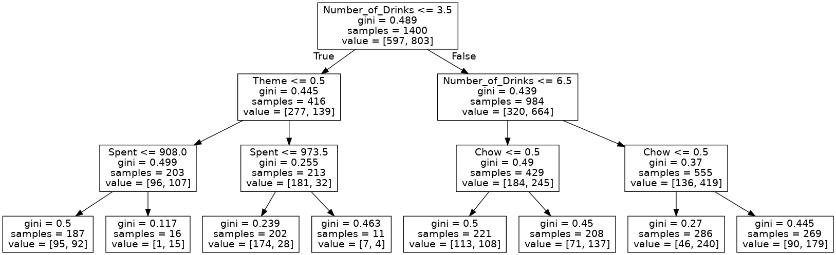
tree.plot_tree(small_tree)
[Text(0.5, 0.875, 'X[1] <= 3.5\ngini = 0.489\nsamples = 1400\nvalue = [597, 803]'),
 Text(0.25, 0.625, 'X[0] <= 0.5\ngini = 0.445\nsamples = 416\nvalue = [277, 139]'),
 Text(0.125, 0.375, 'X[2] <= 908.0\ngini = 0.499\nsamples = 203\nvalue = [96, 107]'),
 Text(0.0625, 0.125, 'gini = 0.5\nsamples = 187\nvalue = [95, 92]'),
 Text(0.1875, 0.125, 'gini = 0.117\nsamples = 16\nvalue = [1, 15]'),
 Text(0.375, 0.375, 'X[2] <= 973.5\ngini = 0.255\nsamples = 213\nvalue = [181, 32]'),
 Text(0.3125, 0.125, 'gini = 0.239\nsamples = 202\nvalue = [174, 28]'),
 Text(0.4375, 0.125, 'gini = 0.463\nsamples = 11\nvalue = [7, 4]'),
 Text(0.75, 0.625, 'X[1] <= 6.5\ngini = 0.439\nsamples = 984\nvalue = [320, 664]'),
 Text(0.625, 0.375, 'X[3] <= 0.5\ngini = 0.49\nsamples = 429\nvalue = [184, 245]'),
 Text(0.5625, 0.125, 'gini = 0.5\nsamples = 221\nvalue = [113, 108]'),
 Text(0.6875, 0.125, 'gini = 0.45\nsamples = 208\nvalue = [71, 137]'),
 Text(0.875, 0.375, 'X[3] <= 0.5\ngini = 0.37\nsamples = 555\nvalue = [136, 419]'),
 Text(0.8125, 0.125, 'gini = 0.27\nsamples = 286\nvalue = [46, 240]'),
 Text(0.9375, 0.125, 'gini = 0.445\nsamples = 269\nvalue = [90, 179]')]

Export tree and convert to a picture file.
dot_data_2 = export_graphviz(small_tree, out_file='small_tree_2.dot', feature_names = train_X.columns)
Looks much better!
predProb_train_2 = small_tree.predict_proba(train_X)
predProb_train_2
array([[0.50802139, 0.49197861],
       [0.16083916, 0.83916084],
       [0.16083916, 0.83916084],
       ...,
       [0.34134615, 0.65865385],
       [0.51131222, 0.48868778],
       [0.51131222, 0.48868778]])
predProb_train_2_df = pd.DataFrame(predProb_train_2, columns = small_tree.classes_)
predProb_train_2_df
| 0 | 1 | |
|---|---|---|
| 0 | 0.508021 | 0.491979 |
| 1 | 0.160839 | 0.839161 |
| 2 | 0.160839 | 0.839161 |
| 3 | 0.861386 | 0.138614 |
| 4 | 0.334572 | 0.665428 |
| ... | ... | ... |
| 1395 | 0.508021 | 0.491979 |
| 1396 | 0.160839 | 0.839161 |
| 1397 | 0.341346 | 0.658654 |
| 1398 | 0.511312 | 0.488688 |
| 1399 | 0.511312 | 0.488688 |
1400 rows × 2 columns
predProb_valid_2 = small_tree.predict_proba(valid_X)
predProb_valid_2
array([[0.33457249, 0.66542751],
       [0.51131222, 0.48868778],
       [0.50802139, 0.49197861],
       ...,
       [0.86138614, 0.13861386],
       [0.16083916, 0.83916084],
       [0.16083916, 0.83916084]])
predProb_valid_2_df = pd.DataFrame(predProb_valid_2, columns = small_tree.classes_)
predProb_valid_2_df
| 0 | 1 | |
|---|---|---|
| 0 | 0.334572 | 0.665428 |
| 1 | 0.511312 | 0.488688 |
| 2 | 0.508021 | 0.491979 |
| 3 | 0.511312 | 0.488688 |
| 4 | 0.334572 | 0.665428 |
| ... | ... | ... |
| 595 | 0.861386 | 0.138614 |
| 596 | 0.511312 | 0.488688 |
| 597 | 0.861386 | 0.138614 |
| 598 | 0.160839 | 0.839161 |
| 599 | 0.160839 | 0.839161 |
600 rows × 2 columns
train_y_pred_2 = small_tree.predict(train_X)
train_y_pred
array([0, 1, 1, ..., 1, 0, 1], dtype=int64)
valid_y_pred_2 = small_tree.predict(valid_X)
valid_y_pred
array([1, 0, 0, 1, 1, 0, 0, 1, 1, 0, 1, 0, 0, 0, 1, 0, 0, 1, 0, 0, 1, 1,
       0, 0, 0, 0, 1, 0, 1, 1, 0, 1, 0, 1, 0, 1, 1, 1, 1, 1, 1, 1, 0, 1,
       1, 0, 1, 1, 1, 0, 0, 0, 0, 0, 1, 0, 1, 0, 1, 0, 0, 0, 1, 0, 1, 1,
       1, 0, 1, 0, 1, 0, 1, 0, 1, 0, 1, 1, 0, 1, 1, 1, 1, 0, 1, 0, 1, 0,
       0, 1, 1, 1, 1, 1, 1, 0, 1, 1, 1, 1, 1, 0, 1, 0, 0, 1, 1, 0, 1, 1,
       0, 1, 1, 0, 1, 1, 0, 0, 1, 0, 1, 0, 0, 1, 0, 1, 1, 1, 1, 0, 1, 0,
       1, 0, 0, 0, 0, 1, 0, 1, 1, 1, 0, 1, 0, 0, 1, 1, 1, 0, 0, 0, 1, 1,
       0, 0, 1, 0, 1, 0, 1, 0, 0, 1, 1, 1, 1, 0, 0, 0, 0, 0, 0, 1, 1, 1,
       1, 0, 1, 1, 1, 0, 1, 0, 0, 0, 1, 0, 0, 0, 1, 1, 0, 1, 0, 1, 1, 0,
       1, 1, 1, 1, 1, 0, 0, 1, 0, 1, 0, 1, 0, 1, 1, 0, 1, 0, 0, 1, 1, 0,
       1, 1, 0, 1, 1, 1, 1, 1, 0, 1, 0, 1, 0, 0, 1, 0, 1, 1, 0, 0, 1, 1,
       1, 1, 1, 1, 0, 1, 0, 1, 0, 1, 1, 1, 0, 1, 1, 0, 0, 1, 0, 1, 0, 0,
       1, 0, 1, 1, 1, 0, 0, 0, 0, 0, 1, 1, 0, 0, 1, 1, 0, 0, 0, 0, 1, 0,
       0, 0, 1, 0, 1, 0, 1, 1, 1, 0, 0, 0, 1, 1, 1, 0, 0, 0, 1, 0, 0, 1,
       0, 1, 0, 0, 1, 1, 1, 0, 0, 1, 1, 1, 0, 1, 1, 1, 1, 0, 1, 1, 1, 1,
       1, 0, 1, 0, 0, 0, 1, 0, 1, 0, 1, 0, 1, 1, 1, 1, 1, 0, 1, 1, 1, 0,
       1, 1, 0, 1, 0, 0, 0, 1, 0, 1, 0, 1, 0, 1, 0, 0, 0, 0, 1, 1, 0, 1,
       0, 1, 1, 1, 1, 0, 0, 0, 0, 0, 0, 1, 0, 0, 1, 0, 0, 1, 1, 1, 0, 1,
       1, 0, 1, 0, 0, 1, 1, 1, 0, 1, 0, 1, 1, 0, 1, 1, 0, 0, 0, 1, 1, 0,
       0, 1, 1, 1, 0, 0, 0, 1, 1, 0, 1, 1, 1, 1, 1, 1, 1, 1, 1, 1, 0, 0,
       1, 1, 0, 1, 1, 0, 1, 1, 0, 1, 1, 0, 0, 1, 0, 1, 1, 0, 1, 0, 1, 0,
       1, 0, 1, 0, 1, 1, 1, 1, 0, 0, 0, 0, 0, 1, 0, 0, 0, 1, 0, 1, 1, 0,
       0, 0, 0, 0, 1, 0, 1, 0, 0, 0, 0, 1, 0, 1, 1, 0, 0, 0, 0, 1, 0, 1,
       1, 1, 1, 0, 0, 1, 1, 1, 1, 1, 1, 1, 0, 0, 0, 1, 1, 0, 1, 0, 1, 1,
       0, 0, 0, 1, 1, 1, 0, 0, 0, 0, 1, 1, 1, 1, 1, 1, 1, 1, 1, 1, 0, 1,
       1, 0, 1, 1, 1, 1, 1, 1, 1, 1, 0, 1, 1, 0, 1, 0, 0, 0, 1, 1, 1, 0,
       1, 0, 0, 1, 0, 1, 1, 1, 1, 0, 0, 0, 0, 0, 0, 0, 0, 0, 1, 1, 1, 1,
       0, 0, 1, 0, 0, 0], dtype=int64)
Confusion matrix.
from sklearn.metrics import confusion_matrix, accuracy_score
Training set.
confusion_matrix_train_2 = confusion_matrix(train_y, train_y_pred_2)
confusion_matrix_train_2
array([[389, 208],
       [232, 571]], dtype=int64)
# from sklearn.metrics import confusion_matrix, ConfusionMatrixDisplay
# import matplotlib.pyplot as plt

confusion_matrix_train_2_display = ConfusionMatrixDisplay(confusion_matrix_train_2, display_labels = small_tree.classes_)
confusion_matrix_train_2_display.plot()
plt.grid(False)

accuracy_train = accuracy_score(train_y, train_y_pred_2)
accuracy_train
0.6857142857142857
from sklearn.metrics import classification_report

print(classification_report(train_y, train_y_pred_2))
              precision    recall  f1-score   support

           0       0.63      0.65      0.64       597
           1       0.73      0.71      0.72       803

    accuracy                           0.69      1400
   macro avg       0.68      0.68      0.68      1400
weighted avg       0.69      0.69      0.69      1400
Cross validation.
from sklearn.model_selection import cross_val_score
from sklearn.model_selection import KFold
import numpy as np
kf = KFold(n_splits = 10)
scores = cross_val_score(estimator = small_tree, X = train_X, y = train_y, cv = kf)
scores
array([0.70714286, 0.7       , 0.57142857, 0.69285714, 0.69285714,
       0.73571429, 0.7       , 0.67857143, 0.6       , 0.68571429])
scores.mean()
0.6764285714285714
Validation set.
from sklearn.metrics import confusion_matrix, accuracy_score

confusion_matrix_valid = confusion_matrix(valid_y, valid_y_pred_2)
confusion_matrix_valid
array([[156,  98],
       [109, 237]], dtype=int64)
accuracy_valid = accuracy_score(valid_y, valid_y_pred_2)
accuracy_valid
0.655
from sklearn.metrics import classification_report

print(classification_report(valid_y, valid_y_pred_2))
              precision    recall  f1-score   support

           0       0.59      0.61      0.60       254
           1       0.71      0.68      0.70       346

    accuracy                           0.66       600
   macro avg       0.65      0.65      0.65       600
weighted avg       0.66      0.66      0.66       600
Change cutoff to 0.7
New confusion matrix for the training set
train_y_pred_2_df = pd.DataFrame(train_y_pred_2, columns = ["pred_50"])
train_y_pred_2_df
| pred_50 | |
|---|---|
| 0 | 0 |
| 1 | 1 |
| 2 | 1 |
| 3 | 0 |
| 4 | 1 |
| ... | ... |
| 1395 | 0 |
| 1396 | 1 |
| 1397 | 1 |
| 1398 | 0 |
| 1399 | 0 |
1400 rows × 1 columns
predProb_train_2_df
| 0 | 1 | |
|---|---|---|
| 0 | 0.508021 | 0.491979 |
| 1 | 0.160839 | 0.839161 |
| 2 | 0.160839 | 0.839161 |
| 3 | 0.861386 | 0.138614 |
| 4 | 0.334572 | 0.665428 |
| ... | ... | ... |
| 1395 | 0.508021 | 0.491979 |
| 1396 | 0.160839 | 0.839161 |
| 1397 | 0.341346 | 0.658654 |
| 1398 | 0.511312 | 0.488688 |
| 1399 | 0.511312 | 0.488688 |
1400 rows × 2 columns
import numpy as np
train_y_pred_2_df["pred_70"] = np.where(predProb_train_2_df.iloc[:, 1] >= 0.7,
                                                     1, 0)
train_y_pred_2_df.head()
| pred_50 | pred_70 | |
|---|---|---|
| 0 | 0 | 0 |
| 1 | 1 | 1 |
| 2 | 1 | 1 |
| 3 | 0 | 0 |
| 4 | 1 | 0 |
Confusion matrix for training set with new cutoff
confusion_matrix_train_2_70 = confusion_matrix(train_y, train_y_pred_2_df["pred_70"])
confusion_matrix_train_2_70
array([[550,  47],
       [548, 255]], dtype=int64)
confusion_matrix_train_2_70_display = ConfusionMatrixDisplay(confusion_matrix_train_2_70,
                                                               display_labels = small_tree.classes_)
confusion_matrix_train_2_70_display.plot()
plt.grid(False)

from sklearn.metrics import classification_report

print(classification_report(train_y, train_y_pred_2_df["pred_70"]))
              precision    recall  f1-score   support

           0       0.50      0.92      0.65       597
           1       0.84      0.32      0.46       803

    accuracy                           0.57      1400
   macro avg       0.67      0.62      0.56      1400
weighted avg       0.70      0.57      0.54      1400
New confusion matrix for the validation set
valid_y_pred_2_df = pd.DataFrame(valid_y_pred_2, columns = ["pred_50"])
valid_y_pred_2_df
| pred_50 | |
|---|---|
| 0 | 1 |
| 1 | 0 |
| 2 | 0 |
| 3 | 0 |
| 4 | 1 |
| ... | ... |
| 595 | 0 |
| 596 | 0 |
| 597 | 0 |
| 598 | 1 |
| 599 | 1 |
600 rows × 1 columns
predProb_valid_2_df
| 0 | 1 | |
|---|---|---|
| 0 | 0.334572 | 0.665428 |
| 1 | 0.511312 | 0.488688 |
| 2 | 0.508021 | 0.491979 |
| 3 | 0.511312 | 0.488688 |
| 4 | 0.334572 | 0.665428 |
| ... | ... | ... |
| 595 | 0.861386 | 0.138614 |
| 596 | 0.511312 | 0.488688 |
| 597 | 0.861386 | 0.138614 |
| 598 | 0.160839 | 0.839161 |
| 599 | 0.160839 | 0.839161 |
600 rows × 2 columns
import numpy as np
valid_y_pred_2_df["pred_70"] = np.where(predProb_valid_2_df.iloc[:, 1] >= 0.7,
                                                     1, 0)
valid_y_pred_2_df.head()
| pred_50 | pred_70 | |
|---|---|---|
| 0 | 1 | 0 |
| 1 | 0 | 0 |
| 2 | 0 | 0 |
| 3 | 0 | 0 |
| 4 | 1 | 0 |
Confusion matrix for validation set with new cutoff
confusion_matrix_valid_2_70 = confusion_matrix(valid_y, valid_y_pred_2_df["pred_70"])
confusion_matrix_valid_2_70
array([[231,  23],
       [233, 113]], dtype=int64)
confusion_matrix_valid_2_70_display = ConfusionMatrixDisplay(confusion_matrix_valid_2_70,
                                                               display_labels = small_tree.classes_)
confusion_matrix_valid_2_70_display.plot()
plt.grid(False)

from sklearn.metrics import classification_report

print(classification_report(valid_y, valid_y_pred_2_df["pred_70"]))
              precision    recall  f1-score   support

           0       0.50      0.91      0.64       254
           1       0.83      0.33      0.47       346

    accuracy                           0.57       600
   macro avg       0.66      0.62      0.56       600
weighted avg       0.69      0.57      0.54       600
ROC using the original cutoff
from sklearn import metrics
import matplotlib.pyplot as plt
from sklearn.metrics import roc_curve
fpr2, tpr2, thresh2 = roc_curve(valid_y, predProb_valid_2[:,1])
import matplotlib.pyplot as plt
plt.style.use("seaborn")

plt.plot(fpr2, tpr2, linestyle = '-', color = "green", label = "Small Tree")

# roc curve for tpr = fpr (random line)
random_probs = [0 for i in range(len(valid_y))]

p_fpr, p_tpr, _ = roc_curve(valid_y, random_probs)

plt.plot(p_fpr, p_tpr, linestyle = '--', color = "black", label = "Random")

# If desired
plt.legend(loc = "best")

plt.title("Small Tree ROC")

plt.xlabel("False Positive Rate")

plt.ylabel("True Positive Rate");

# to save the plot
# plt.savefig("whatever_name",dpi = 300)

from sklearn.metrics import roc_auc_score
auc2 = roc_auc_score(valid_y, predProb_valid_2[:,1])
auc2
0.7259569432433662
from sklearn.model_selection import GridSearchCV
param_grid = {"max_depth": [3, 5, 10],
             "min_samples_split": [15, 25, 35],
              "min_impurity_decrease": [0, 0.005, 0.001]}
grid_search = GridSearchCV(DecisionTreeClassifier(random_state = 666), param_grid, cv = 10)
grid_search_fit = grid_search.fit(train_X, train_y)
grid_search_fit
GridSearchCV(cv=10, estimator=DecisionTreeClassifier(random_state=666),
             param_grid={'max_depth': [3, 5, 10],
                         'min_impurity_decrease': [0, 0.005, 0.001],
                         'min_samples_split': [15, 25, 35]})
print(grid_search.best_score_)
0.6814285714285715
print(grid_search.best_params_)
{'max_depth': 10, 'min_impurity_decrease': 0.001, 'min_samples_split': 35}
best_tree = grid_search.best_estimator_
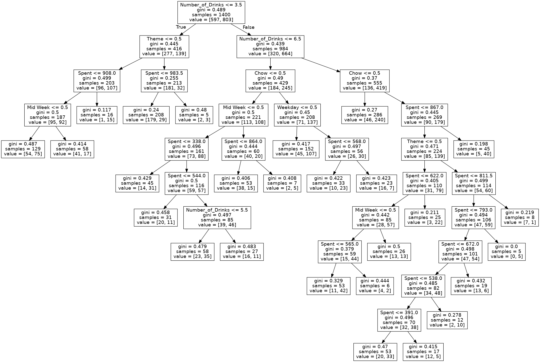
tree.plot_tree(best_tree)
[Text(0.435, 0.9545454545454546, 'X[1] <= 3.5\ngini = 0.489\nsamples = 1400\nvalue = [597, 803]'),
 Text(0.2, 0.8636363636363636, 'X[0] <= 0.5\ngini = 0.445\nsamples = 416\nvalue = [277, 139]'),
 Text(0.12, 0.7727272727272727, 'X[2] <= 908.0\ngini = 0.499\nsamples = 203\nvalue = [96, 107]'),
 Text(0.08, 0.6818181818181818, 'X[4] <= 0.5\ngini = 0.5\nsamples = 187\nvalue = [95, 92]'),
 Text(0.04, 0.5909090909090909, 'gini = 0.487\nsamples = 129\nvalue = [54, 75]'),
 Text(0.12, 0.5909090909090909, 'gini = 0.414\nsamples = 58\nvalue = [41, 17]'),
 Text(0.16, 0.6818181818181818, 'gini = 0.117\nsamples = 16\nvalue = [1, 15]'),
 Text(0.28, 0.7727272727272727, 'X[2] <= 983.5\ngini = 0.255\nsamples = 213\nvalue = [181, 32]'),
 Text(0.24, 0.6818181818181818, 'gini = 0.24\nsamples = 208\nvalue = [179, 29]'),
 Text(0.32, 0.6818181818181818, 'gini = 0.48\nsamples = 5\nvalue = [2, 3]'),
 Text(0.67, 0.8636363636363636, 'X[1] <= 6.5\ngini = 0.439\nsamples = 984\nvalue = [320, 664]'),
 Text(0.5, 0.7727272727272727, 'X[3] <= 0.5\ngini = 0.49\nsamples = 429\nvalue = [184, 245]'),
 Text(0.4, 0.6818181818181818, 'X[4] <= 0.5\ngini = 0.5\nsamples = 221\nvalue = [113, 108]'),
 Text(0.32, 0.5909090909090909, 'X[2] <= 338.0\ngini = 0.496\nsamples = 161\nvalue = [73, 88]'),
 Text(0.28, 0.5, 'gini = 0.429\nsamples = 45\nvalue = [14, 31]'),
 Text(0.36, 0.5, 'X[2] <= 544.0\ngini = 0.5\nsamples = 116\nvalue = [59, 57]'),
 Text(0.32, 0.4090909090909091, 'gini = 0.458\nsamples = 31\nvalue = [20, 11]'),
 Text(0.4, 0.4090909090909091, 'X[1] <= 5.5\ngini = 0.497\nsamples = 85\nvalue = [39, 46]'),
 Text(0.36, 0.3181818181818182, 'gini = 0.479\nsamples = 58\nvalue = [23, 35]'),
 Text(0.44, 0.3181818181818182, 'gini = 0.483\nsamples = 27\nvalue = [16, 11]'),
 Text(0.48, 0.5909090909090909, 'X[2] <= 864.0\ngini = 0.444\nsamples = 60\nvalue = [40, 20]'),
 Text(0.44, 0.5, 'gini = 0.406\nsamples = 53\nvalue = [38, 15]'),
 Text(0.52, 0.5, 'gini = 0.408\nsamples = 7\nvalue = [2, 5]'),
 Text(0.6, 0.6818181818181818, 'X[5] <= 0.5\ngini = 0.45\nsamples = 208\nvalue = [71, 137]'),
 Text(0.56, 0.5909090909090909, 'gini = 0.417\nsamples = 152\nvalue = [45, 107]'),
 Text(0.64, 0.5909090909090909, 'X[2] <= 568.0\ngini = 0.497\nsamples = 56\nvalue = [26, 30]'),
 Text(0.6, 0.5, 'gini = 0.422\nsamples = 33\nvalue = [10, 23]'),
 Text(0.68, 0.5, 'gini = 0.423\nsamples = 23\nvalue = [16, 7]'),
 Text(0.84, 0.7727272727272727, 'X[3] <= 0.5\ngini = 0.37\nsamples = 555\nvalue = [136, 419]'),
 Text(0.8, 0.6818181818181818, 'gini = 0.27\nsamples = 286\nvalue = [46, 240]'),
 Text(0.88, 0.6818181818181818, 'X[2] <= 867.0\ngini = 0.445\nsamples = 269\nvalue = [90, 179]'),
 Text(0.84, 0.5909090909090909, 'X[0] <= 0.5\ngini = 0.471\nsamples = 224\nvalue = [85, 139]'),
 Text(0.76, 0.5, 'X[2] <= 622.0\ngini = 0.405\nsamples = 110\nvalue = [31, 79]'),
 Text(0.72, 0.4090909090909091, 'X[4] <= 0.5\ngini = 0.442\nsamples = 85\nvalue = [28, 57]'),
 Text(0.68, 0.3181818181818182, 'X[2] <= 565.0\ngini = 0.379\nsamples = 59\nvalue = [15, 44]'),
 Text(0.64, 0.22727272727272727, 'gini = 0.329\nsamples = 53\nvalue = [11, 42]'),
 Text(0.72, 0.22727272727272727, 'gini = 0.444\nsamples = 6\nvalue = [4, 2]'),
 Text(0.76, 0.3181818181818182, 'gini = 0.5\nsamples = 26\nvalue = [13, 13]'),
 Text(0.8, 0.4090909090909091, 'gini = 0.211\nsamples = 25\nvalue = [3, 22]'),
 Text(0.92, 0.5, 'X[2] <= 811.5\ngini = 0.499\nsamples = 114\nvalue = [54, 60]'),
 Text(0.88, 0.4090909090909091, 'X[2] <= 793.0\ngini = 0.494\nsamples = 106\nvalue = [47, 59]'),
 Text(0.84, 0.3181818181818182, 'X[2] <= 672.0\ngini = 0.498\nsamples = 101\nvalue = [47, 54]'),
 Text(0.8, 0.22727272727272727, 'X[2] <= 538.0\ngini = 0.485\nsamples = 82\nvalue = [34, 48]'),
 Text(0.76, 0.13636363636363635, 'X[2] <= 391.0\ngini = 0.496\nsamples = 70\nvalue = [32, 38]'),
 Text(0.72, 0.045454545454545456, 'gini = 0.47\nsamples = 53\nvalue = [20, 33]'),
 Text(0.8, 0.045454545454545456, 'gini = 0.415\nsamples = 17\nvalue = [12, 5]'),
 Text(0.84, 0.13636363636363635, 'gini = 0.278\nsamples = 12\nvalue = [2, 10]'),
 Text(0.88, 0.22727272727272727, 'gini = 0.432\nsamples = 19\nvalue = [13, 6]'),
 Text(0.92, 0.3181818181818182, 'gini = 0.0\nsamples = 5\nvalue = [0, 5]'),
 Text(0.96, 0.4090909090909091, 'gini = 0.219\nsamples = 8\nvalue = [7, 1]'),
 Text(0.92, 0.5909090909090909, 'gini = 0.198\nsamples = 45\nvalue = [5, 40]')]

dot_data_3 = export_graphviz(best_tree, out_file='best_tree_3.dot', feature_names = train_X.columns)
predProb_train_3 = best_tree.predict_proba(train_X)
predProb_train_3
array([[0.41860465, 0.58139535],
       [0.16083916, 0.83916084],
       [0.16083916, 0.83916084],
       ...,
       [0.29605263, 0.70394737],
       [0.59259259, 0.40740741],
       [0.59259259, 0.40740741]])
pd.DataFrame(predProb_train_3, columns = best_tree.classes_)
| 0 | 1 | |
|---|---|---|
| 0 | 0.418605 | 0.581395 |
| 1 | 0.160839 | 0.839161 |
| 2 | 0.160839 | 0.839161 |
| 3 | 0.860577 | 0.139423 |
| 4 | 0.500000 | 0.500000 |
| ... | ... | ... |
| 1395 | 0.418605 | 0.581395 |
| 1396 | 0.160839 | 0.839161 |
| 1397 | 0.296053 | 0.703947 |
| 1398 | 0.592593 | 0.407407 |
| 1399 | 0.592593 | 0.407407 |
1400 rows × 2 columns
predProb_valid_3 = best_tree.predict_proba(valid_X)
predProb_valid_3
array([[0.5       , 0.5       ],
       [0.71698113, 0.28301887],
       [0.41860465, 0.58139535],
       ...,
       [0.86057692, 0.13942308],
       [0.16083916, 0.83916084],
       [0.16083916, 0.83916084]])
pd.DataFrame(predProb_valid_3, columns = best_tree.classes_)
| 0 | 1 | |
|---|---|---|
| 0 | 0.500000 | 0.500000 |
| 1 | 0.716981 | 0.283019 |
| 2 | 0.418605 | 0.581395 |
| 3 | 0.645161 | 0.354839 |
| 4 | 0.377358 | 0.622642 |
| ... | ... | ... |
| 595 | 0.860577 | 0.139423 |
| 596 | 0.396552 | 0.603448 |
| 597 | 0.860577 | 0.139423 |
| 598 | 0.160839 | 0.839161 |
| 599 | 0.160839 | 0.839161 |
600 rows × 2 columns
train_y_pred_3 = best_tree.predict(train_X)
train_y_pred_3
array([1, 1, 1, ..., 1, 0, 0], dtype=int64)
valid_y_pred_3 = best_tree.predict(valid_X)
valid_y_pred_3
array([0, 0, 1, 0, 1, 1, 1, 0, 1, 0, 1, 0, 0, 1, 1, 0, 1, 0, 1, 0, 1, 0,
       1, 1, 1, 1, 1, 0, 1, 1, 1, 1, 1, 1, 0, 1, 1, 1, 1, 1, 1, 1, 1, 0,
       1, 1, 1, 1, 1, 1, 1, 0, 0, 1, 0, 0, 1, 1, 1, 0, 0, 1, 1, 0, 1, 0,
       1, 1, 1, 0, 1, 0, 1, 1, 1, 0, 0, 1, 1, 1, 1, 1, 1, 1, 1, 0, 1, 0,
       1, 1, 1, 1, 0, 0, 1, 0, 1, 1, 1, 1, 0, 0, 1, 1, 0, 1, 1, 0, 1, 1,
       0, 1, 1, 1, 1, 0, 0, 1, 1, 0, 0, 0, 1, 1, 1, 1, 1, 1, 1, 0, 1, 1,
       1, 0, 1, 1, 0, 1, 1, 1, 1, 1, 0, 1, 1, 0, 1, 1, 0, 1, 0, 0, 1, 1,
       1, 1, 1, 1, 1, 0, 1, 0, 1, 1, 1, 1, 1, 1, 1, 1, 0, 0, 0, 0, 1, 1,
       1, 1, 0, 1, 1, 1, 0, 1, 1, 1, 1, 1, 0, 1, 1, 0, 0, 1, 1, 0, 1, 0,
       1, 0, 1, 1, 1, 0, 0, 1, 0, 1, 1, 1, 1, 0, 1, 0, 1, 1, 1, 1, 1, 0,
       1, 1, 0, 1, 1, 1, 1, 0, 0, 1, 1, 1, 1, 0, 0, 1, 1, 1, 1, 1, 1, 1,
       1, 1, 1, 1, 1, 1, 1, 1, 0, 1, 1, 0, 1, 1, 1, 0, 1, 1, 1, 1, 0, 0,
       1, 1, 1, 1, 0, 0, 0, 0, 0, 1, 1, 0, 1, 0, 1, 1, 0, 0, 0, 1, 1, 0,
       1, 1, 1, 1, 1, 0, 0, 1, 1, 1, 0, 1, 0, 1, 1, 1, 1, 1, 1, 1, 1, 1,
       1, 1, 0, 1, 1, 1, 1, 0, 1, 0, 1, 1, 1, 1, 1, 1, 0, 1, 1, 0, 1, 0,
       1, 1, 1, 1, 0, 0, 1, 0, 1, 1, 1, 0, 1, 0, 1, 1, 1, 0, 1, 1, 0, 0,
       0, 1, 0, 1, 1, 0, 0, 1, 1, 1, 1, 1, 0, 1, 1, 1, 0, 0, 1, 1, 1, 1,
       1, 1, 1, 1, 0, 0, 0, 1, 0, 1, 1, 1, 0, 1, 1, 0, 0, 0, 1, 1, 1, 1,
       0, 1, 1, 0, 0, 1, 1, 1, 0, 1, 0, 1, 1, 0, 1, 1, 0, 0, 1, 1, 1, 0,
       0, 1, 0, 0, 0, 0, 0, 1, 1, 1, 1, 1, 1, 1, 1, 1, 1, 0, 1, 1, 1, 0,
       1, 1, 1, 1, 1, 0, 1, 1, 0, 1, 1, 0, 1, 1, 0, 1, 1, 0, 1, 0, 1, 0,
       1, 1, 1, 1, 1, 1, 1, 1, 0, 1, 0, 0, 1, 1, 0, 0, 1, 1, 1, 1, 1, 0,
       1, 1, 1, 1, 1, 0, 0, 0, 0, 0, 0, 1, 1, 1, 1, 1, 0, 0, 1, 1, 0, 1,
       1, 1, 1, 1, 0, 1, 1, 0, 1, 1, 1, 1, 0, 0, 0, 1, 1, 0, 0, 0, 1, 1,
       0, 1, 0, 1, 1, 1, 0, 0, 1, 1, 1, 1, 1, 1, 1, 1, 0, 1, 1, 1, 0, 1,
       1, 1, 1, 1, 1, 1, 1, 0, 1, 1, 1, 1, 0, 0, 1, 1, 1, 1, 1, 0, 1, 0,
       1, 1, 1, 1, 1, 1, 1, 1, 1, 0, 1, 0, 1, 0, 0, 0, 0, 0, 1, 1, 1, 1,
       0, 0, 1, 0, 1, 1], dtype=int64)
Confusion matrix.
from sklearn.metrics import confusion_matrix, accuracy_score
Training set.
confusion_matrix_train_3 = confusion_matrix(train_y, train_y_pred_3)
confusion_matrix_train_3
array([[359, 238],
       [117, 686]], dtype=int64)
# from sklearn.metrics import confusion_matrix, ConfusionMatrixDisplay
# import matplotlib.pyplot as plt

confusion_matrix_train_3_display = ConfusionMatrixDisplay(confusion_matrix_train_3, display_labels = best_tree.classes_)
confusion_matrix_train_3_display.plot()
plt.grid(False)

accuracy_train = accuracy_score(train_y, train_y_pred_3)
accuracy_train
0.7464285714285714
from sklearn.metrics import classification_report

print(classification_report(train_y, train_y_pred_3))
              precision    recall  f1-score   support

           0       0.75      0.60      0.67       597
           1       0.74      0.85      0.79       803

    accuracy                           0.75      1400
   macro avg       0.75      0.73      0.73      1400
weighted avg       0.75      0.75      0.74      1400
Cross validation.
from sklearn.model_selection import cross_val_score
from sklearn.model_selection import KFold
import numpy as np
kf = KFold(n_splits = 10)
scores = cross_val_score(estimator = best_tree, X = train_X, y = train_y, cv = kf)
scores
array([0.68571429, 0.65714286, 0.65      , 0.65      , 0.69285714,
       0.71428571, 0.62857143, 0.70714286, 0.67142857, 0.72857143])
scores.mean()
0.6785714285714286
Validation set.
from sklearn.metrics import confusion_matrix, accuracy_score

confusion_matrix_valid_3 = confusion_matrix(valid_y, valid_y_pred_3)
confusion_matrix_valid_3
array([[125, 129],
       [ 66, 280]], dtype=int64)
# from sklearn.metrics import confusion_matrix, ConfusionMatrixDisplay
# import matplotlib.pyplot as plt

confusion_matrix_valid_3_display = ConfusionMatrixDisplay(confusion_matrix_valid_3, display_labels = best_tree.classes_)
confusion_matrix_valid_3_display.plot()
plt.grid(False)

accuracy_valid = accuracy_score(valid_y, valid_y_pred_3)
accuracy_valid
0.675
from sklearn.metrics import classification_report

print(classification_report(valid_y, valid_y_pred_3))
              precision    recall  f1-score   support

           0       0.65      0.49      0.56       254
           1       0.68      0.81      0.74       346

    accuracy                           0.68       600
   macro avg       0.67      0.65      0.65       600
weighted avg       0.67      0.68      0.67       600
ROC.
from sklearn import metrics
import matplotlib.pyplot as plt
from sklearn.metrics import roc_curve
fpr3, tpr3, thresh3 = roc_curve(valid_y, predProb_valid_3[:,1])
import matplotlib.pyplot as plt
plt.style.use("seaborn")

plt.plot(fpr3, tpr3, linestyle = '-', color = "purple", label = "Best Tree")

# roc curve for tpr = fpr (random line)
random_probs = [0 for i in range(len(valid_y))]

p_fpr, p_tpr, _ = roc_curve(valid_y, random_probs)

plt.plot(p_fpr, p_tpr, linestyle = '--', color = "black", label = "Random")

# If desired
plt.legend()

plt.title("Best Tree")

plt.xlabel("False Positive Rate")

plt.ylabel("True Positive Rate");

# to save the plot
# plt.savefig("whatever_name",dpi = 300)

from sklearn.metrics import roc_auc_score
auc3 = roc_auc_score(valid_y, predProb_valid_3[:,1])
auc3
0.7146579582176505
from sklearn.ensemble import RandomForestClassifier

rf = RandomForestClassifier(max_depth = 10, random_state = 666)
rf.fit(train_X, train_y)
RandomForestClassifier(max_depth=10, random_state=666)
train_y_pred_rf = rf.predict(train_X)
train_y_pred_rf
array([1, 1, 1, ..., 1, 0, 1], dtype=int64)
valid_y_pred_rf = rf.predict(valid_X)
valid_y_pred_rf
array([1, 0, 1, 1, 1, 1, 1, 0, 1, 1, 1, 0, 0, 0, 1, 0, 1, 0, 1, 0, 1, 0,
       1, 0, 0, 1, 1, 0, 1, 1, 1, 1, 1, 1, 1, 1, 1, 1, 1, 1, 1, 1, 1, 1,
       1, 1, 1, 1, 1, 0, 1, 0, 0, 0, 1, 0, 1, 0, 1, 1, 0, 1, 1, 0, 1, 1,
       1, 1, 1, 0, 1, 0, 1, 1, 1, 0, 0, 1, 0, 1, 1, 1, 1, 1, 1, 0, 1, 0,
       0, 1, 1, 1, 1, 1, 1, 0, 1, 0, 1, 1, 1, 1, 1, 1, 0, 1, 1, 0, 1, 1,
       0, 1, 1, 1, 1, 1, 0, 0, 1, 0, 1, 0, 1, 1, 0, 1, 1, 1, 1, 0, 1, 1,
       1, 0, 1, 1, 0, 0, 0, 1, 1, 1, 0, 0, 1, 1, 1, 0, 1, 0, 0, 1, 1, 1,
       1, 0, 1, 1, 1, 0, 1, 1, 0, 1, 1, 1, 1, 1, 1, 0, 1, 0, 0, 1, 1, 0,
       1, 1, 1, 1, 1, 1, 0, 1, 1, 0, 1, 1, 0, 0, 1, 0, 1, 0, 1, 1, 1, 0,
       0, 0, 1, 1, 1, 0, 0, 1, 0, 0, 0, 1, 1, 1, 1, 0, 0, 0, 0, 1, 1, 0,
       1, 1, 0, 1, 1, 1, 1, 0, 0, 1, 1, 1, 1, 0, 0, 0, 1, 1, 0, 0, 1, 1,
       1, 1, 1, 1, 1, 1, 1, 0, 1, 1, 1, 0, 1, 1, 1, 0, 0, 1, 1, 1, 0, 0,
       1, 1, 0, 1, 0, 0, 0, 0, 0, 0, 1, 0, 1, 0, 1, 1, 0, 0, 1, 1, 1, 1,
       0, 1, 1, 0, 1, 0, 0, 1, 1, 1, 0, 1, 1, 0, 1, 1, 1, 0, 1, 0, 1, 1,
       1, 1, 0, 1, 1, 1, 1, 1, 0, 1, 1, 1, 1, 1, 1, 1, 0, 0, 1, 0, 1, 1,
       1, 0, 1, 0, 0, 0, 1, 0, 0, 1, 1, 0, 1, 1, 1, 1, 1, 1, 1, 1, 1, 0,
       1, 1, 1, 1, 0, 0, 0, 0, 1, 1, 0, 1, 0, 1, 0, 0, 1, 0, 1, 1, 0, 1,
       1, 1, 0, 1, 1, 0, 0, 0, 0, 1, 0, 1, 0, 1, 0, 0, 0, 0, 1, 1, 1, 1,
       0, 0, 1, 0, 0, 1, 1, 1, 0, 1, 0, 1, 1, 0, 1, 1, 1, 0, 1, 1, 1, 0,
       0, 1, 0, 0, 0, 0, 0, 1, 0, 1, 1, 1, 1, 0, 1, 1, 1, 0, 1, 1, 1, 0,
       1, 1, 0, 1, 1, 0, 0, 1, 0, 1, 1, 0, 0, 1, 0, 1, 1, 0, 1, 0, 1, 0,
       1, 0, 1, 0, 0, 1, 1, 1, 0, 1, 0, 0, 1, 1, 0, 1, 0, 1, 1, 1, 1, 0,
       1, 1, 1, 1, 1, 0, 1, 0, 0, 0, 0, 1, 0, 1, 1, 1, 0, 0, 0, 1, 0, 1,
       1, 1, 1, 0, 0, 1, 1, 1, 1, 1, 1, 1, 0, 0, 1, 1, 1, 0, 1, 1, 1, 1,
       0, 0, 1, 1, 1, 1, 0, 0, 1, 1, 1, 0, 1, 1, 1, 1, 1, 1, 1, 1, 0, 1,
       1, 0, 1, 1, 1, 1, 1, 0, 1, 1, 1, 1, 1, 0, 1, 1, 1, 0, 1, 0, 1, 0,
       1, 1, 1, 1, 0, 1, 0, 1, 1, 0, 1, 0, 0, 0, 0, 0, 0, 0, 1, 1, 1, 1,
       0, 0, 0, 0, 1, 1], dtype=int64)
var_importance = rf.feature_importances_
var_importance
array([0.06023784, 0.32952713, 0.50781572, 0.04724778, 0.02935665,
       0.02581488])
std = np.std([tree.feature_importances_ for tree in
   rf.estimators_], axis = 0)
std
array([0.02612911, 0.05569014, 0.04720133, 0.0230609 , 0.01441775,
       0.0128291 ])
var_importance_df = pd.DataFrame({"variable": train_X.columns, "importance": var_importance, "std": std})
var_importance_df
| variable | importance | std | |
|---|---|---|---|
| 0 | Theme | 0.060238 | 0.026129 |
| 1 | Number_of_Drinks | 0.329527 | 0.055690 |
| 2 | Spent | 0.507816 | 0.047201 |
| 3 | Chow | 0.047248 | 0.023061 |
| 4 | Mid Week | 0.029357 | 0.014418 |
| 5 | Weekday | 0.025815 | 0.012829 |
var_importance_df.sort_values("importance")
| variable | importance | std | |
|---|---|---|---|
| 5 | Weekday | 0.025815 | 0.012829 |
| 4 | Mid Week | 0.029357 | 0.014418 |
| 3 | Chow | 0.047248 | 0.023061 |
| 0 | Theme | 0.060238 | 0.026129 |
| 1 | Number_of_Drinks | 0.329527 | 0.055690 |
| 2 | Spent | 0.507816 | 0.047201 |
var_importance_plot = var_importance_df.plot(kind = "barh", xerr = "std", x = "variable", legend=False)
var_importance_plot.set_ylabel("")
var_importance_plot.set_xlabel("Importance")
plt.show()

confusion_matrix_train_rf = confusion_matrix(train_y, train_y_pred_rf)
confusion_matrix_train_rf
array([[519,  78],
       [ 22, 781]], dtype=int64)
# from sklearn.metrics import confusion_matrix, ConfusionMatrixDisplay
# import matplotlib.pyplot as plt

confusion_matrix_train_rf_display = ConfusionMatrixDisplay(confusion_matrix_train_rf, display_labels = rf.classes_)
confusion_matrix_train_rf_display.plot()
plt.grid(False)

# from sklearn.metrics import classification_report

print(classification_report(train_y, train_y_pred_rf))
              precision    recall  f1-score   support

           0       0.96      0.87      0.91       597
           1       0.91      0.97      0.94       803

    accuracy                           0.93      1400
   macro avg       0.93      0.92      0.93      1400
weighted avg       0.93      0.93      0.93      1400
confusion_matrix_valid_rf = confusion_matrix(valid_y, valid_y_pred_rf)
confusion_matrix_valid_rf
array([[129, 125],
       [ 91, 255]], dtype=int64)
# from sklearn.metrics import confusion_matrix, ConfusionMatrixDisplay
# import matplotlib.pyplot as plt

confusion_matrix_valid_rf_display = ConfusionMatrixDisplay(confusion_matrix_valid_rf, display_labels = rf.classes_)
confusion_matrix_valid_rf_display.plot()
plt.grid(False)

# from sklearn.metrics import classification_report

print(classification_report(valid_y, valid_y_pred_rf))
              precision    recall  f1-score   support

           0       0.59      0.51      0.54       254
           1       0.67      0.74      0.70       346

    accuracy                           0.64       600
   macro avg       0.63      0.62      0.62       600
weighted avg       0.64      0.64      0.64       600
predProb_valid_rf = rf.predict_proba(valid_X)
predProb_valid_rf
array([[0.19484426, 0.80515574],
       [0.61708693, 0.38291307],
       [0.37797144, 0.62202856],
       ...,
       [0.83796426, 0.16203574],
       [0.17397095, 0.82602905],
       [0.07917024, 0.92082976]])
predProb_valid_rf_df = pd.DataFrame(predProb_valid_rf, columns = rf.classes_)
predProb_valid_rf_df
| 0 | 1 | |
|---|---|---|
| 0 | 0.194844 | 0.805156 |
| 1 | 0.617087 | 0.382913 |
| 2 | 0.377971 | 0.622029 |
| 3 | 0.087739 | 0.912261 |
| 4 | 0.114974 | 0.885026 |
| ... | ... | ... |
| 595 | 0.858953 | 0.141047 |
| 596 | 0.653956 | 0.346044 |
| 597 | 0.837964 | 0.162036 |
| 598 | 0.173971 | 0.826029 |
| 599 | 0.079170 | 0.920830 |
600 rows × 2 columns
# from sklearn import metrics
# import matplotlib.pyplot as plt
# from sklearn.metrics import roc_curve

fpr4, tpr4, thresh4 = roc_curve(valid_y, predProb_valid_rf[:,1])
import matplotlib.pyplot as plt
plt.style.use("seaborn")

plt.plot(fpr4, tpr4, linestyle = '-', color = "orange", label = "Random Forest")

# roc curve for tpr = fpr (random line)
random_probs = [0 for i in range(len(valid_y))]

p_fpr, p_tpr, _ = roc_curve(valid_y, random_probs)

plt.plot(p_fpr, p_tpr, linestyle = '--', color = "purple", label = "Random")

# If desired
plt.legend()

plt.title("Random Forest ROC")

plt.xlabel("False Positive Rate")

plt.ylabel("True Positive Rate");

# to save the plot
# plt.savefig("whatever_name",dpi = 300)

# from sklearn.metrics import roc_auc_score

auc4 = roc_auc_score(valid_y, predProb_valid_rf[:,1])
auc4
0.6912407264120888
Combining all the ROCs
import matplotlib.pyplot as plt
plt.style.use("seaborn")

plt.plot(fpr1, tpr1, linestyle = "-", color = "blue", label = "Full Tree")
plt.plot(fpr2, tpr2, linestyle = "-", color = "green", label = "Small Tree")
plt.plot(fpr3, tpr3, linestyle = "-", color = "purple", label = "Best Tree")
plt.plot(fpr4, tpr4, linestyle = "-", color = "orange", label = "Random Forest")


# roc curve for tpr = fpr (random line)
random_probs = [0 for i in range(len(valid_y))]

p_fpr_random, p_tpr_random, _ = roc_curve(valid_y, random_probs, pos_label = 1)

plt.plot(p_fpr_random, p_tpr_random, linestyle = "--", color = "black", label = "Random")

# If desired
plt.legend()

plt.title("Decision Tree Hangover ROC")

plt.xlabel("False Positive Rate")

plt.ylabel("True Positive Rate");

# to save the plot
# plt.savefig("whatever_name",dpi = 300)

print(auc1, auc2, auc3, auc4)
0.571042510582131 0.7259569432433662 0.7146579582176505 0.6912407264120888
data = {"Full Tree": auc1, "Small Tree": auc2, "Best Tree" : auc3, "Random Forest": auc4}

auc_df = pd.DataFrame([data])
auc_df
| Full Tree | Small Tree | Best Tree | Random Forest | |
|---|---|---|---|---|
| 0 | 0.571043 | 0.725957 | 0.714658 | 0.691241 |
class_tr_new = pd.read_csv("hangover_new_data.csv")
class_tr_new
| Theme | Number_of_Drinks | Spent | Chow | Mid Week | Weekday | |
|---|---|---|---|---|---|---|
| 0 | 0 | 6 | 666 | 1 | 0 | 0 |
predProb_class_tr_new_1 = best_tree.predict_proba(class_tr_new)
predProb_class_tr_new_1
array([[0.29605263, 0.70394737]])
predProb_class_tr_new_1_df = pd.DataFrame(predProb_class_tr_new_1, columns = best_tree.classes_)
predProb_class_tr_new_1_df
| 0 | 1 | |
|---|---|---|
| 0 | 0.296053 | 0.703947 |
new_pred_1 = best_tree.predict(class_tr_new)
new_pred_1
array([1], dtype=int64)
new_pred_1_df = pd.DataFrame(new_pred_1, columns = ["Best_Tree_Prediction "])
new_pred_1_df
| Best_Tree_Prediction | |
|---|---|
| 0 | 1 |
Change cutoff to 0.7
import numpy as np
new_pred_1_df["Best_Tree_Prediction_70"] = np.where(predProb_class_tr_new_1_df.iloc[:, 1] >= 0.7,
                                                     1, 0)
new_pred_1_df.head()
| Best_Tree_Prediction | Best_Tree_Prediction_70 | |
|---|---|---|
| 0 | 1 | 1 |

predProb_class_tr_new_rf = rf.predict_proba(class_tr_new)
predProb_class_tr_new_rf
array([[0.21611204, 0.78388796]])
predProb_class_tr_new_rf_df = pd.DataFrame(predProb_class_tr_new_rf, columns = rf.classes_)
predProb_class_tr_new_rf_df
| 0 | 1 | |
|---|---|---|
| 0 | 0.216112 | 0.783888 |
rf_new_pred = rf.predict(class_tr_new)
rf_new_pred
array([1], dtype=int64)
rf_new_pred_df = pd.DataFrame(rf_new_pred, columns = ["RF_Prediction"])
rf_new_pred_df
| RF_Prediction | |
|---|---|
| 0 | 1 |
Change cutoff to 0.7
import numpy as np
rf_new_pred_df["Best_Tree_Prediction_70"] = np.where(predProb_class_tr_new_rf_df.iloc[:, 1] >= 0.7,
                                                     1, 0)
rf_new_pred_df.head()
| RF_Prediction | Best_Tree_Prediction_70 | |
|---|---|---|
| 0 | 1 | 1 |
It's time to retrace your steps... HEH HEH HEH HEH HEH :-)